OlmoEarth v1.3 Turns Planetary Imagery Into Reusable Features

Satellite analysis often begins with a deceptively expensive step: turning large stacks of imagery into features a model can use. Ai2’s OlmoEarth v1.3 release changes that starting point. Instead of requiring every project to process raw imagery or fine-tune a foundation model immediately, it offers a model plus precomputed annual embeddings that can support lighter downstream experiments.

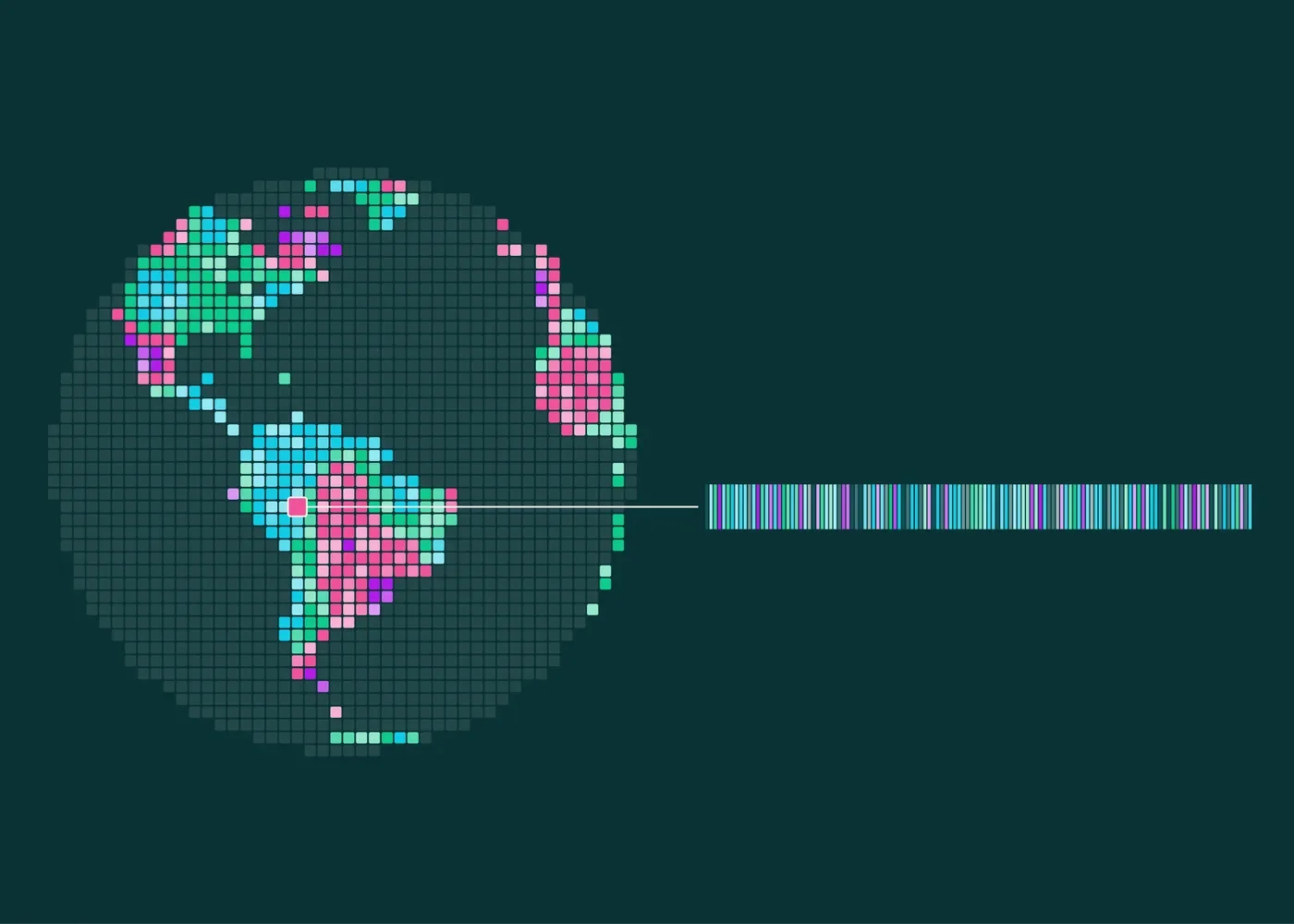
The release announcement says OlmoEarth reads annual time series from Sentinel-1 radar, Sentinel-2 multispectral imagery, and Landsat. It produces a 128-number vector for each 10-meter pixel, with the first 64 dimensions usable as a smaller representation. Ai2 has also published global embeddings through Source Cooperative and introduced a browser-based Embeddings Explorer.

That combination matters more than any single benchmark number. It gives practitioners a staged workflow: explore a signal, validate it against imagery and labels, train a small task-specific model, and only then decide whether custom embedding generation or full fine-tuning is justified.

What a reusable planetary embedding changes

An embedding is not a finished crop, fire, mining, or land-cover map. It is a compact representation that places information from several observations into a feature vector. A downstream classifier can learn how those features relate to a specific label set. Change analysis can also compare vectors from different years to identify locations worth closer inspection.

This separates expensive representation learning from cheaper task learning. Consider a team mapping three land-cover classes in one district. The team can label a modest sample, train a lightweight classifier over the published vectors, inspect its errors, and revise the labels without repeatedly decoding a year of satellite scenes. A second team studying a different question can reuse the same vectors with its own labels.

The smaller 64-dimensional option introduces a useful engineering choice. Halving the feature width can reduce storage, transfer, and downstream compute, but teams should test whether that economy preserves performance for their geography and classes. The announcement reports that the 128-dimensional embeddings ranked highest overall across 27 evaluations and led 20 of them, while the 64-dimensional representation led 18. Those aggregate results are encouraging, but they do not guarantee the best result on a new local task.

A practical evaluation ladder

The explorer can shorten the distance between a question and a first visual check. Users can navigate a false-color embedding map, compare years, inspect Sentinel-2 imagery, search for similar places, add labeled points, train a small classifier, and export a GeoTIFF. This is a useful screening environment, not a substitute for a defensible validation process.

A sensible evaluation can proceed in four stages:

1. Define the target precisely. “Forest change” could mean canopy loss, seasonal variation, fire damage, plantation harvest, or sensor artifacts. The label definition should match the decision the map will support.
2. Separate training and testing geographically. Randomly splitting nearby pixels can overstate performance because neighboring observations share landscape and acquisition conditions. Holding out entire regions offers a harder test of transfer.
3. Inspect imagery and provenance. A high embedding difference indicates change in the representation, not its cause. Cloud, phenology, flooding, cultivation cycles, or input coverage may explain the signal. The release says provenance tables identify source scenes for each 20-kilometer tile and year, enabling this audit.
4. Compare with a simple baseline. A lightweight model using a few conventional spectral or temporal features can reveal whether the embedding adds enough value to justify additional storage and complexity.

Accuracy should also be reported per class and region. A strong average can conceal poor recall for rare events or systematic errors in landscapes absent from the training labels. For monitoring uses, teams should decide whether missed events or false alarms carry the larger operational cost.

Coverage and resolution are real boundaries

The archive is substantial, but it is not a uniform historical record. At launch, the announcement describes global coverage for 2023, 2024, and 2025, while embeddings from 2017 through 2022 cover selected countries. A project requiring consistent annual comparison across a decade must therefore confirm that every needed place and year is available.

A 10-meter pixel is also not equivalent to a 10-meter ground truth object. Mixed pixels can combine roads, vegetation, roofs, soil, and water. Small structures or narrow disturbances may not dominate the representation. Conversely, a classifier can produce crisp-looking boundaries that imply more certainty than its inputs support. Output maps should retain confidence information where possible and state the effective spatial and temporal limits.

Annual embeddings are well suited to broad year-over-year questions, but they may smooth over short events or seasonal timing. If the relevant signal depends on a particular month, crop stage, storm, or acquisition window, generating embeddings for custom dates may be more appropriate than relying on annual products. Radar and optical sources also have different sensitivities, so investigators should connect a detected pattern back to the underlying imagery before assigning a physical explanation.

When to move beyond the precomputed vectors

Precomputed embeddings are a strong first choice when the goal is rapid feasibility testing, regional classification, similarity search, or annual change triage. They reduce infrastructure demands and let domain experts spend more time refining labels and error criteria.

Custom generation becomes relevant when a project needs unavailable years, a narrower time window, different input modalities, or tighter control over resolution and preprocessing. Fine-tuning may be worthwhile when a well-labeled task consistently exposes information the generic representation does not capture. Neither step should be automatic: evidence from held-out evaluation should justify the added compute and maintenance burden.

OlmoEarth v1.3 is therefore best understood as reusable geospatial infrastructure rather than a universal mapping answer. Its model, published vectors, provenance records, and interactive tooling make serious experimentation more accessible. The quality of the resulting map still depends on clear labels, representative validation, source-image review, and honest limits on what an embedding can establish.