A Forecast Is More Than a Number: Evaluating Granite PatchTST-FM-r2

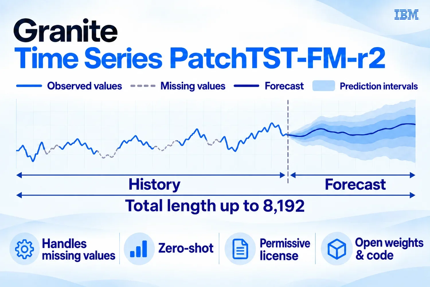
IBM introduced Granite Time Series PatchTST-FM-r2 on September 9, 2026. Its announcement describes a roughly 385-million-parameter forecasting model with open weights, probabilistic predictions and support for filling missing values. IBM also publishes its implementation and benchmark reproduction material, offering Apache 2.0 or OpenMDW 1.0 licensing.

The release is worth examining because forecasting is not simply another form of text generation. A fluent sentence can look plausible without being correct; a smooth forecast line can create the same illusion. The practical question is whether the forecast supports a better decision than an inexpensive alternative. That requires a test designed around your actual operating conditions, rather than a screenshot of a leaderboard.

Start with the decision, not the model

Consider an illustrative shop deciding how much stock to order for next week. Ordering too little loses sales, while ordering too much ties up cash and may create waste. Those two mistakes need not have equal costs. A forecast that minimises average numerical error might still recommend an unsuitable inventory policy if it repeatedly underestimates the busiest days.

Write down the decision before preparing data: what will change when the forecast changes, how far ahead must the decision be made, and which mistakes are expensive? A staffing application may need hourly forecasts several days ahead. A maintenance application may care more about unusual excursions than average demand. These are different evaluation problems even if both begin with timestamped numbers.

Then establish a simple baseline. Repeat the last observed value, or use the corresponding period from the previous week where seasonality makes that reasonable. These baselines are not embarrassing competitors. They reveal how much useful signal a more complicated system actually adds and remain practical fallbacks when infrastructure fails.

Preserve the arrow of time

Randomly splitting observations can leak future information into a forecasting test. Instead, choose historical cutoffs. At each cutoff, provide only information available at that moment and compare the resulting forecast with what happened afterward. Repeat this procedure across quiet periods, holidays, outages and changing demand patterns.

Feature preparation must obey the same rule. A cleaned dataset can accidentally include corrections that were applied days later. Likewise, a promotional calendar may be available in advance while actual customer attendance is not. Record when each input became available, not merely the date it describes. Otherwise a successful offline test may be measuring privileged access to the future.

Missing observations deserve their own policy. A missing sensor reading is not automatically zero activity. Distinguish an absent measurement from a genuine zero, and check how each case changes the forecast. Keep the original missingness information during evaluation so that data repairs do not conceal the conditions under which the model struggles.

Ask whether uncertainty is useful

A probability distribution is valuable only when it changes a decision sensibly. In the shop example, the median forecast might support routine replenishment, while a higher demand quantile could inform a more conservative stock policy. The correct choice depends on business costs, not on a universal preference for a particular percentile.

Check coverage as well as accuracy. If an interval is intended to capture most outcomes, measure how often outcomes actually fall inside it. Repeat that measurement by product group and forecast horizon. An interval that works well on average may systematically miss demand spikes or become unreliable further into the future.

Do not assume that a wide interval is useless. Sometimes it correctly reflects limited information. The useful response may be a smaller commitment, a human review or a shorter planning horizon. Pretending uncertainty does not exist does not make the underlying decision less risky.

Make deployment an experiment with a stopping rule

Run the candidate in shadow mode before allowing it to change orders or staffing. Log inputs, forecasts, runtime and the action that would have followed. Compare those proposed actions with the existing process. This separates prediction quality from the effect of changing a business rule at the same time.

Decide in advance what would justify adoption and what would trigger rollback. Include data freshness, operational latency and failure handling alongside predictive metrics. Preserve a versioned model and evaluation dataset so that a later regression can be investigated. The strongest outcome is not merely a better-looking forecast: it is a repeatable improvement in decisions, with an understandable fallback when conditions change.