What a Zero-Token Judge Changes About Confidence-Based Evaluation

Automated judges are often prompted to produce a verdict, explanation, and confidence score as text. Darwin-27B-ZTC takes a different route: it treats judging as classification and returns a probability distribution over the allowed answers without generating an answer sequence. The distinction matters most when confidence will drive an operational decision, such as accepting an answer automatically or escalating it for review.

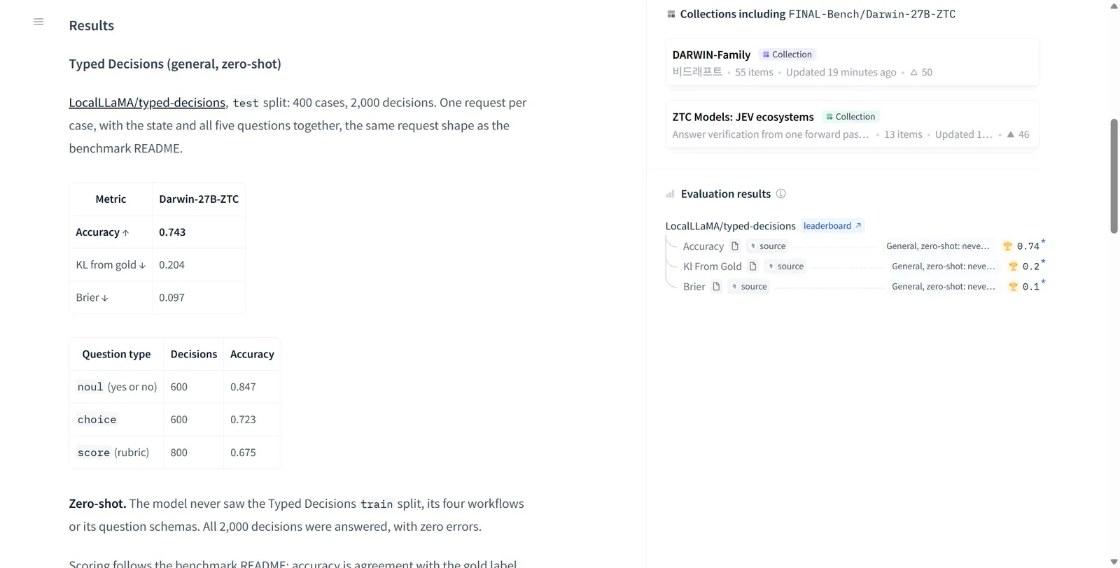
The model's authors report 0.743 overall accuracy on 2,000 judgments from the general split of the typed-decisions benchmark in a zero-shot setting. They also report a Brier score of 0.097 and KL divergence of 0.204. Those figures are useful starting points, but deploying a judge requires understanding what each number can—and cannot—establish.

From verdict generation to probability estimation

A conventional generative judge receives a prompt and decodes tokens until it has expressed a decision. Even when the desired output is just a label, the system must constrain or parse generated text. Confidence may come from token log probabilities, repeated samples, or a second self-assessment prompt. Each method introduces choices about formatting, sampling, and aggregation.

A classifier-style judge instead defines the valid outcomes in advance and assigns probability mass across them. For a binary question, an output might be {correct: 0.82, incorrect: 0.18}. For a multiple-choice task, the same pattern extends over the candidate options. This makes the contract between model and application clearer: downstream code receives a typed distribution rather than prose that must be interpreted.

Calling the approach “zero-token” does not mean computation is free. The model still performs a forward pass over its input, and input length, batch size, hardware, and serving implementation still affect latency and cost. The narrower claim is that it avoids autoregressive output decoding. That can remove a variable portion of the work, especially when the alternative emits lengthy rationales, but real throughput should be measured on the intended stack.

Why calibration belongs beside accuracy

Accuracy asks how often the top-ranked answer is right. Calibration asks whether stated probabilities match observed frequencies. Imagine two judges that are each correct on 80 of 100 cases. If one assigns roughly 80% confidence to that group while the other routinely claims 99%, they have the same accuracy but very different risk profiles.

The difference becomes concrete in a routing policy. Suppose items above a confidence threshold are accepted automatically and everything else goes to a human. An overconfident judge can send difficult, incorrect cases through the automatic path. A conservative judge may be safer but create too much review work. Choosing the threshold therefore requires both discrimination—the ability to rank easier cases above harder ones—and reliable probabilities.

Brier score summarizes squared error between predicted probabilities and observed outcomes, with lower values indicating better performance under the chosen formulation. KL divergence is another distribution-sensitive summary. Neither scalar reveals where errors occur. Two systems with similar aggregate scores may behave differently in their highest-confidence region, which is usually the region an auto-accept policy relies on most.

Reading the benchmark by task type

The reported per-type accuracies are 0.847 for free-form correctness (noul), 0.723 for candidate selection (choice), and 0.675 for scoring (score). The spread warns against treating the overall figure as a universal judge quality number. Each response type poses a different decision problem, and a workload with mostly ordinal scoring may behave unlike the benchmark aggregate.

A practical evaluation should preserve these slices and add ones that reflect the application: subject area, prompt length, language, model family, safety severity, and ambiguous versus clear-cut cases. For ordinal scores, exact-match accuracy can also hide whether mistakes are adjacent or extreme. Mean absolute error, rank correlation, or a task-specific cost matrix may provide a more useful companion metric.

The authors describe deterministic outputs for identical inputs, which removes sampling variation from decoding. Reproducibility still depends on the surrounding system. Changes to model weights, numerical precision, inference kernels, preprocessing, prompt templates, or label definitions can alter results. Versioning those elements is essential if a threshold is expected to remain stable.

A deployment checklist for confidence gates

Start with a held-out sample drawn from the actual traffic distribution, not only the public benchmark. Plot observed accuracy against predicted confidence in fixed or equal-frequency bins, and inspect the bins around the proposed threshold. Report sample counts as well as rates; a seemingly clean high-confidence bin may contain too few examples to support a policy.

Next, compare policies rather than only models. Measure coverage at each threshold, error rate among automatically accepted items, and the fraction sent for review. For asymmetric applications, attach a larger cost to dangerous false accepts than to unnecessary escalations. Select the operating point from that cost curve.

Finally, repeat the analysis under plausible shifts: new source models, longer prompts, novel domains, and adversarial inputs. Calibration measured on one distribution does not automatically transfer to another. Monitor accepted-item error and confidence histograms after launch, while retaining a sampled human-review stream that can reveal silent drift.

Darwin-27B-ZTC presents a clean architectural proposition: a judge can expose its decision distribution directly instead of wrapping classification inside generation. Its published results make that proposition testable. The next step for any adopter is not to inherit the headline threshold, but to establish whether the probabilities remain useful on the exact decisions, costs, and shifts of the intended system.