SlideOn Turns Retrieval Knowledge Into Searchable Sparse Features
LightOn’s SlideOn and mSlideOn explore a practical middle path in neural search: convert dense or late-interaction token representations into learned sparse features that can be served through an inverted index.


Sparse conversion can reuse a capable retriever while changing its indexing economics, but the right pruning point must be measured on the target corpus and serving stack.
Search systems usually force an architectural choice early. Dense retrieval compresses each document into a fixed-width vector and searches a nearest-neighbor index. Late interaction retains multiple token vectors and scores their cross-document matches, preserving more detail at additional cost. Sparse retrieval instead emits a mostly empty vector whose active dimensions can be served through posting lists, much like a traditional inverted index.
LightOn’s SlideOn and mSlideOn releases make that third option more interesting because they do not begin from an untrained sparse representation. They start with knowledge already present in dense and late-interaction retrievers, then use sparse autoencoders and retrieval fine-tuning to produce indexable sparse features. SlideOn is the English-focused 174-million-parameter model derived from DenseOn; mSlideOn is a 339-million-parameter multilingual model derived from mLateOn. The announcement also provides model checkpoints, intermediate autoencoder checkpoints, training data references, and training and evaluation scripts.
Why sparse representations change the serving problem
A dense index compares a query vector with candidate vectors in a continuous space. Approximate-nearest-neighbor methods make that practical, but operators still need to choose an index structure, compression settings, and often specialized acceleration. A sparse index organizes documents by active feature. When a query activates a feature, the engine visits only that feature’s posting list and accumulates scores for the documents it finds there. Documents with no shared active features can be skipped.
That difference shifts the main operating budget. Instead of only asking how many dense dimensions a model produces, teams need to measure how many sparse features are active per query and document, how long their posting lists become, and how aggressively features can be pruned. Two models with the same latent vocabulary size may therefore have very different storage and latency profiles. The useful unit is not simply model parameters or embedding width; it is the entire encode, index, retrieve, and rerank path.
Sparse neural features also differ from ordinary term-frequency indexes. A learned feature can respond to a concept expressed with different words, potentially reducing lexical mismatch. The tradeoff is interpretability: a tokenizer-vocabulary dimension has an obvious label, while an autoencoder latent may require examples and probing before its behavior is understandable. That matters in applications where search administrators must explain why a result matched or enforce rules tied to literal terms.
What the conversion recipe contributes
The release uses a sparse autoencoder as a bridge between an existing retriever and a sparse index. At a high level, the encoder maps each contextual token representation into a much larger latent space, keeps only its strongest activations, and the decoder learns to reconstruct the original representation. This reconstruction phase encourages the sparse features to retain information already learned by the starting model. Supervised retrieval fine-tuning then adapts those features for ranking rather than reconstruction alone.
This division of labor is valuable. Autoencoder training supplies a latent dictionary without repeating full retrieval pretraining, while supervised fine-tuning can correct the mismatch between “reconstruct this vector” and “rank the relevant document first.” It also provides a reusable experimental pattern: compare the frozen starting retriever, the autoencoder-only representation, and the fully fine-tuned sparse model. Those checkpoints reveal whether gains come from knowledge transfer, the sparse bottleneck, or task supervision.
The authors use a 32,768-feature latent space and Top-K selection during autoencoder pretraining. They also train for pruning robustness, allowing an operator to retain fewer activations when storage or latency is tighter. These values are design choices, not universal defaults. Corpus size, document length, language distribution, and the index implementation can all move the best operating point.
Reading the reported results carefully
The release reports 56.68 on BEIR-15 for SlideOn versus 56.20 for DenseOn. For mSlideOn, it reports improvements over mDenseOn of 4.76 points on MIRACL and 10.19 points on MLDR, as well as gains on the cited code-retrieval evaluation. Those comparisons support the authors’ claim that their sparse conversion preserves useful retrieval knowledge, but they do not establish the same advantage for every production corpus.
Benchmark averages can hide important variation. A multilingual average may combine languages with very different training coverage, tokenization behavior, and document lengths. Long-document benchmarks may reward preserving signals that are rare in short passages. Code search may depend on exact identifiers as well as semantic intent. Before adoption, teams should inspect per-dataset and per-language results and reproduce the intended pruning configuration rather than transferring the headline score directly.
It is equally important to distinguish encoder quality from system performance. A model can improve ranking metrics while producing posting lists that are expensive for a particular engine. Conversely, modest pruning may sharply reduce index size without materially changing quality. Measurements should include encoding throughput, mean and tail query latency, index build time, index bytes per document, active features per vector, and recall or ranking quality at each pruning level.
A practical evaluation plan
Start with a representative corpus snapshot and a query set containing navigational, semantic, rare-term, multilingual, and long-document cases. Keep document segmentation and relevance judgments fixed across BM25, the current dense or late-interaction baseline, and the sparse candidate. This prevents chunking changes from masquerading as model improvements.
Next, build several sparse indexes with progressively stricter pruning. Record quality and serving cost at each point, then plot the Pareto frontier rather than selecting the highest-quality run automatically. Inspect failure cases for three distinct problems: missing concepts at encoding time, overly aggressive feature removal, and ranking errors among retrieved candidates. Each points to a different remedy.
Finally, test hybrid behavior. Literal identifiers, names, and numbers may still benefit from a lexical signal, while learned sparse features can help with paraphrases. A weighted combination or staged retrieval pipeline may be more reliable than replacing an established lexical system outright. SlideOn and mSlideOn are best understood as new components for this design space: they make pretrained neural retrieval knowledge compatible with inverted-index mechanics, while leaving the final quality, transparency, and cost balance to corpus-specific evaluation.
Source: SlideOn & mSlideOn: Sparsified Late-Interaction and Dense Retrievers ↗. How we write